IntroductionAndroid and iOS are underlying operating systems used in mobile technology. Android is a technology given by Google and iOS introduced by Apple. Both technologies have certain pros & cons. However Android being preferred by most manufacturers is the most popular smartphone platform. SimilaritiesAndroid and iOS are fairly similar considering the user interface. Interfaces give touching capabilities like tapping swiping etc. Android giving customization capability makes it more flexible than iOS, but iOS is user friendly. Similar status bars giving information like battery life, Wi-Fi, cell signals etc. while Android exploring more information like new messages, emails and reminders. Android ensures security by isolating apps from other resources of the system unless user gives the accessibility to the system resources. IOS ensures the security by reviewing apps and verifying the identity of publishers. DifferencesAndroid devices have more variety in shapes, prices and hardware proficiencies, whereas iOS is only available on Apple devices like iPhones and iPods. Android uses Chrome as its browser whereas iOS uses Safari. From app building and publishing point of view Android is enhanced than iOS since it is an open source i.e. anyone can download and make Android apps (free or paid) using freely available SDK and upload them on Google Play store. Google charges a one-time 25$ fee from developers who want to publish their apps while iOS developers pay 99$ yearly for using iOS SDK and publishing apps on Apple’s App store. Programming languages used for Android development are C, C++ and java, whereas iOS apps are build-in Objective-C. ConclusionConcluding all this discussion both OS have their own set of values. But keeping in mind that Android is an open source, flexible, customizable and having variety in hardware devices, Android is lot more well than iOS.
0 Comments
The main distinctive feature of mobile communications system is the combination of communication with mobility. The evolution process of wireless and mobile communication is very fast. We’ve reached the fourth generation (4G) of wireless access technologies in a relatively short span of time. The first generation (1G) fulfilled the basic mobile voice, second generation (2G) implemented features like capacity and coverage, third and fourth generations (3G & 4G) actually implemented higher data rates or high speed availability of wireless access technologies.
1G mobile technology systems were available in 1980 and used analog radio transmission techniques to provide simple voice services.1G used frequency division multiplexing technique (FDMA) which has certain limitations. 2G refers to digital systems providing services like short messaging and low speed data transmission. Some 2G technologies include CDMA2000 1xRTT and GSM. 2G technologies were available in 1990. 2G used either time division multiplexing (TDMA) or code multiplexing techniques. 3G technology requirements were specified by ITU as a project named as International Mobile Telephone 2000 (IMT-2000). Some primary 3G technologies include UMTS-HSPA and CDMA2000 EV-DO also WIMAX has been recently designated as official 3G technology. 3G technologies start emerging in the last decade. 4G technology requirement has also been specified by ITU as IMT-Advanced with relatively higher data rates. In 4G technology, all previously available services would also be include like, GSM Global System for Mobile Communication, GPRS General Packet Radio Service, IMT-2000 International Mobile Communications, Wi-fi Wireless Fidelity, and Blutooth. Due to the immense interest of customers in wireless and mobile communication technologies, we see that this technology has grown in a relatively small period of time. Starting from basic mobile conversations (1G) to add a lot more services with higher data rates and also to combine all previous features will bring a very interesting and a revolutionary era in the form of 4G technology. Introduction: Microprocessor also called CPU (central processing unit) or logic chip is the core of a computer. It is the main computational device which do all arithmatic, logical and control calculations. These tasks are performed by using digital logic design steps on microprocessors. In 1971 first intel microprocessor was developed which made the architecture of computers a lot more simple. Instruction set, bandwidth and clock speed are the parameters to differentiate different processors. Architecture: The main things in the architecture of Intel 8085 microprocessor are memory, interrupts, I/O ports, registers, instruction sets and addressing modes. The total memory used in intel 8085 microprocessor for addressing is 64 KB. Jump and data in microprocessor are controlled by 16 bit addresses. Size of memory control the limit of stack memory. 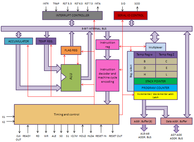
There are mainly five types of interrupts e.g INTR, RST 5.5, RST 6.5, RST 7.5 and Trap. They perform different actions or call different instructions when they are occur ed. They can be enabled or disabled using different instruction sets. Coming back to the architecture of Intel 8085 microprocessor there are 256 input and output ports used for different actions. Eight bit registers are used to perform different operations. Then there are different instructions or commands which are used to perform different actions. Also different kind of addressing modes are used.
Applications: The applications of microprocessors varies from the field of communication and medical to the field of instrumentation. Some applications include credit card processing, ECG, DVD player, telephone exchanges, telephone sets, satellite communication, mobile phone and modems. References: www.computer.howstuffworks.com/microprocessor.htm www.webopedia.com/TERM/M/microprocessor.html www.teachurselfece.com www.zseries.in/embedded%lab/8085%microprocessor/other%applications  Prepared By:
Muhammad Shahzad Instructions: Step1: Download Tools From Given Link: http://www.mediafire.com/download/77ki2j21n3evmly/Frameworks+Fiddler.zip Step2: Run windows powershell (as adminstrator) Step3: Then run this following command. Show-WindowsDeveloperLicenseRegistration Step4: Click agree and log into your microsoft live id.There will be a prompt showing information about your developer license. Then close it. Step5: Again run powershell (not as adminstrator). Step6: Run following command add-appxpackage(give space and drag framework into the powershell, press enter). Repeat the process for all of three frameworks. (Provided frameworks are latest upto march 03, 2014, if they are not updated, you can get them from updated visual studio) Step7: Open fiddler, and go to win 8 config, mark store and save changes.All above process is only for 1st time when you install new window. Step8: To install your apps Run fiddler and go to store and start installation of app, when installation starts, fiddler captures url, now cancel your installation, copy url and paste into idm, download it. (Idm link has resume capability, if it expires(generally it does not), refresh it, use fiddler to capture new link). Step9: Open powershell run the following command. add-appxpackage(space and drag downloaded appx package into powershell, press enter) Note: Important!!! If you have used fiddler in your own laptop, you will be able to run that application, otherwise if your are using on another laptop, it will give error, which can be removed by restarting your laptop after getting developers license, if still, not resolved, in error screen, click on go to store, and then click repair(you must be logged into the store otherwise repair option will not occur) Once it starts installation, cancel it, now you can run application with 100% success. In Isaac Newton's day, one of the biggest problems was poor navigation at sea.Before calculus was developed, the stars were vital for navigation.Shipwrecks occurred because the ship was not where the captain thought it should be. There was not a good enough understanding of how the Earth, stars and planets moved with respect to each other. Calculus (differentiation and integration) was developed to improve this understanding. Differentiation and integration can help us solve many types of real-world problems. We use the derivative to determine the maximum and minimum values of particular functions (e.g. cost, strength, amount of material used in a building, profit, loss, etc.). Derivatives are met in many engineering and science problems, especially when modeling the behavior of moving objects. Our discussion begins with some general applications which we can then apply to specific problems. 1. It is used ECONOMIC a lot, calculus is also a base of economics2.it is used in history, for predicting the life of a stone 3.it is used in geography, which is used to study the gases present in the atmosphere 4. It is mainly used in daily by pilots to measure the pressure n the air. Shipwrecks occurred because the ship was not where the captain thought it should be. There was not a good enough understanding of how the Earth, stars and planets moved with respect to each other. Calculus (differentiation and integration) was developed to improve this understanding. Differentiation and integration can help us solve many types of real-world problems. We use the derivative to determine the maximum and minimum values of particular functions (e.g. cost, strength, amount of material used in a building, profit,loss, etc.). Derivatives are met in many engineering and science problems, especially when modeling the behavior of moving objects. INTEGRATION: 1. Applications of the Indefinite Integral shows how to find displacement (from velocity) and velocity (from acceleration) using the indefinite integral. There are also some electronics applications. In primary school, we learnt how to find areas of shapes with straight sides (e.g. area of a triangle or rectangle). But how do you find areas when the sides are curved? e.g. 2. Area under a Curve and 3. Area in between the two curves. Answer is by Integration. 4. Volume of Solid of Revolution explains how to use integration to find the volume of an object with curved sides, e.g. wine barrels. 5. Centroid of an Area means the cenetr of mass. We see how to use integration to find the centroid of an area with curved sides. 6. Moments of Inertia explain how to find the resistance of a rotating body. We use integration when the shape has curved sides. 7. Work by a Variable Force shows how to find the work done on an object when the force is not constant. 8. Electric Charges have a force between them that varies depending on the amount of charge and the distance between the charges. We use integration to calculate the work done when charges are separated. 9. Average Value of a curve can be calculated using integration. Introduction: Sounds are a part of everyday life. From requisite hearing ability to entertainment in motion pictures and music, sounds have provided the impetus for audio engineers to increase quality of life or level of entertainment through their study and manipulation. In this project, We shall implement a digital sound effects processor; specifically, focusing on basic effects such as, delay, delay with feedback, chorus, and flanger. All these tasks will be simulated using MATLAB. Functions:
Explanations:1). The Delay In its simplest form, a delay effect takes an audio signal and plays it back after a delay time. This “echo deviceâ€, as it is otherwise known, produces a single copy of the input, delayed by anywhere from several microseconds to several seconds. A more interesting sound is produced through the use of feedback control, which takes the output of the delay and sends it back to the input, typically after multiplying by a gain less than or equal to one. This enables the sound to be repeated over and over again, becoming more attenuated with each successive loop. Theoretically, feedback can be used to produce a sound which continues forever, but practically, at some point, the sound level will fall below that of the ambient noise in the system, and the sound will no longer be audible. 2). The Chorus Similar to a chorus of singers, the chorus effect acts to make a single instrument sound like a group of instruments being played. Qualitatively, it is described as adding a thickness to a sound, creating a more lush sound. The chorus effect is reproducing two things: a delay and a difference in pitch between sounds, much like there would be for several instruments playing together. The pitch difference will be generated by storing the sample into larger or smaller memory blocks. In a smaller memory block, the sample is read faster thus increasing the pitch. In a larger memory block, the sample is read slower thus decreasing the pitch. The delay time for chorus is commonly between 20ms and 30ms. The delay time will be varying as well which introduces a problem. Since samples are read in at integral multiples of the sample time, a changing delay time could cause us to require a sample that is not integral. To overcome this problem, we will attempt to use linear interpolation. 3). The Flanger Flanger is much like the chorus, but with a few subtle differences. The flanger also consists of a delay line with varying delay time, but a feedback loop is used as well to generate some distortion in the delayed sound. The common delay for flanger is between 1ms and 10ms which is what gives the input a “whooshing†sound. A low frequency oscillator will be used in this case to control the varying delay line. The same problem will occur here as it did in chorus, so linear interpolation will be used again. Basically, the implementation is similar to chorus, except for a feedback looping and adding to the original signal (see block diagram). 5). The Controls Using Matlab’s GUI, a control panel will be created with slider bars to control the varying effects. For delay, the controls consist of: Delay Rate and Feedback Gain (Delay with Feedback Only.) For chorus, the controls include: Delay Rate and Seed. The seed will be just a seed for the random number generator. For flanger, the controls are: Delay Rate, Low Frequency Output Frequency, and Feedback Gain. For the EQ, the following controls will be needed: Low Band Gain, Mid Band Gain, and High Band Gain. The LFO Frequency will be used to set the frequency at which the delay line is changing. The LFO will be restricted to a range of 0.001Hz and 3.0Hz. The controls will be designed using Matlab’s Build feature which allows you to layout a GUI and add features such as drop down menus, radio buttons, as well as slider bars. Complete Code:Code Of Main Function: clear all; prompt={'Enter wav file path.'}; def={'rec1.wav'}; dlgTitle='Input for wav file'; LineNo=1; answer=inputdlg(prompt,dlgTitle,LineNo,def); out=1; hfile=answer(1); for i = 1:1 file = sprintf('%s%d.wav','rec',i); input('Press enter when ready for recording'); y = wavrecord(88200,44100); soundsc(y,44100); wavwrite(y,44100,file); end [org fs nbits]=wavread('rec1.wav'); while(out) b= menu('Press button to play','actual signal','echo','multiple echo','reverb1','reverb2','reverb3','flanger','pitch_l','pitch_h','fade_in','fade_out','exit'); disp(b); switch(b) case 1, y=org; case 2, y=echo1; case 3, y=mecho1; case 4, y=reverb1; case 5, y=reverb2; case 6, y=reverb3; case 7, y=flanger; case 8, y=pitchshift_l; case 9, y=pitchshift_h; case 10, y=fade_in; case 11, y=fade_out; case 12, out=0; otherwise y=org; end if(out) sound(y,fs); end end Code Of Echo Function: function y=echo1(); [x,fs,nbits]=wavread('rec1.wav'); xlen=length(x); a=0.5; R=ceil(fs*100e-3); y=zeros(size(x)); d=zeros(size(x)); %filter for i=1:1:R+1 y(i)=x(i); end for i=R+1:1:xlen y(i)=x(i)+a*x(i-R); d(i)=a*x(i-R); end Code Of Multiple Echo Function: function y=mecho1(); [x,fs,nbits]=wavread('rec1.wav'); xlen=length(x); a0=0.9; a1=0.8; a2=0.7; R=ceil(fs*120e-3); len=size(x)+3*R; y=zeros(1,len); %filter part x=x'; d0=[zeros(1,R) x zeros(1,2*R)];d0=a0*d0; d1=[zeros(1,2*R) x zeros(1,R)];d1=a1*d1; d2=[zeros(1,3*R) x];d2=a2*d2; for i=1:1:R+1 y(i)=x(i); end y=[x zeros(1,3*R)]+d0+d1+d2; Code Of Reverb Function: There are three functions of Reverb as follows: function y=reverb1(); [d,r,nbits]=wavread('rec1.wav'); noOfSample=r*80e-3 num=[0,zeros(1,noOfSample),1]; den=[1,zeros(1,noOfSample),-0.8]; d1=filter(num,den,d); y=d1; function y=reverb2(); [d,r,nbits]=wavread('rec1.wav'); R=ceil(r*70e-3); num=[0.5,zeros(1,R),1]; den=[1,zeros(1,R),0.5]; d1=filter(num,den,d); y=d1; function y=reverb3(); a1=0.6;a2=0.4;a3=0.2;a4=0.1;a5=0.7;a6=0.6;a7=0.8; R1=700;R2=900;R3=600;R4=400;R5=450;R6=390; [d,r]=wavread('rec1.wav'); num1=[0,zeros(1,R1-1),1]; den1=[1,zeros(1,R1-1),-a1]; d1=filter(num1,den1,d); num2=[0,zeros(1,R2-1),1]; den2=[1,zeros(1,R2-1),-a2]; d2=filter(num2,den2,d); num3=[0,zeros(1,R3-1),1]; den3=[1,zeros(1,R3-1),-a3]; d3=filter(num3,den3,d); num4=[0,zeros(1,R4-1),1]; den4=[1,zeros(1,R4-1),-a4]; d4=filter(num4,den4,d); dIIR=d1+d2+d3+d4; num5=[a5,zeros(1,R5-1),1]; den5=[1,zeros(1,R5-1),a5]; dALL1=filter(num5,den5,dIIR); num5=[1,zeros(1,R6-1),1]; den5=[1,zeros(1,R6-1),a6]; dALL2=filter(num5,den5,dALL1); dTOTAL=d+a7*dALL2; y=dTOTAL; Code Of Flanger Function: function y=flanger(); [x,fs,n]=wavread('rec1.wav'); %sound(x,fs); a=2; delay=10e-3; D=ceil(delay*fs); xlen=length(x); y=zeros(size(x)); %filter for i=1:1:D+1 y(i)=x(i); end for i=D+1:1:xlen delay(i)=abs(round(D*cos(2*pi*i/((xlen-D-1))))); y(i)=x(i)+a*x(i-delay(i)); end Code Of Low Pitch Function: function y=pitchshift_l(); [x,fs,n]=wavread('rec1.wav'); N=length(x); M2=1.5; x_inter=zeros(1,M2*N); x_inter(1:M2:M2*N)=x; y=x_inter; Code Of High Pitch Function: function y=pitchshift_h(); [x,fs,n]=wavread('rec1.wav'); N=length(x); M1=2; x_deci=x(1:M1:N); y=x_deci; Code Of Fade In Function: function y=fade_in(); [yin,fs,nbits]=wavread('rec1.wav'); yin=yin'; step=1/length(yin); fd=0:step:(1-step); fadin=fd.*yin; y=fadin; Code Of Fade Out Function: function y=fade_out(); [yin,fs,nbits]=wavread('rec1.wav'); yin=yin'; step=1/length(yin); fd=1:-step:(0+step); fadout=fd.*yin; y=fadout; TaskDesign a practical integrator using OP_AMP in Multicim. Observe the output for different types of inputs.Integrator AmplifierA circuit in which output voltage is directly proportional to the integral of the input is known as an integrator or the integration amplifier. Such a circuit is obtained by using operational amplifier in the inverting configuration with the feedback resistor RF replaced by a capacitor, CF.Circuit Schematic:
|


 RSS Feed
